Random variable

In mathematics, a random variable (or stochastic variable) is (in general) a measurable function that maps a probability space into a measurable space. Random variables mapping all possible outcomes of an event into the real numbers are frequently studied in elementary statistics and used in the sciences to make predictions based on data obtained from scientific experiments. In addition to scientific applications, random variables were developed for the analysis of games of chance and stochastic events. The utility of random variables comes from their ability to capture only the mathematical properties necessary to answer probabilistic questions.

While the above definition of a random variable requires a familiarity with measure theory to appreciate, the language and structure of random variables can be grasped at various levels of mathematical fluency through limiting the variables one considers. Beyond the introductory level, however, set theory and calculus are fundamental to their study. The concept of a random variable is closely linked to the term "random variate": a random variate is a particular outcome (value) of a random variable.

There are two types of random variables: discrete and continuous.^[1] A discrete random variable maps events to values of a countable set (e.g., the integers), with each value in the range having probability greater than or equal to zero. A continuous random variable maps events to values of an uncountable set (e.g., the real numbers). In a continuous random variable, the probability of any specific value is zero, although the probability of an infinite set of values (such as an interval of non-zero length) may be positive. However, a random variable can be "mixed", having part of its probability spread out over an interval like a typical continuous variable, and part of it concentrated on particular values, like a discrete variable. This categorisation into types is directly equivalent to the categorisation of probability distributions.

A random variable has an associated probability distribution and frequently also a probability density function. Probability density functions are commonly used for continuous variables.

1 Intuitive description
- 1.1 Examples
- 1.2 Non-real-valued form
2 Formal definition
3 Real-valued random variables
- 3.1 Distribution functions of random variables
- 3.2 Moments
4 Functions of random variables
- 4.1 Example 1
- 4.2 Example 2
5 Equivalence of random variables
6 Convergence
7 See also
8 References
- 8.1 Literature

Intuitive description

In the simplest case, a random variable maps events to real numbers. A random variable can be thought of as a function mapping the sample space of a random process to a set of numbers or quantifiable labels.

Examples

For a coin toss, the possible events are heads or tails. The possible outcomes for one fair coin toss can be described using the following random variable:

$X = \begin{cases}head,\\ tail .\end{cases}$

and if the coin is equally likely to land on either side then it has a probability mass function given by:

$\rho_X(x) = \begin{cases}\frac{1}{2},& \text{if }x=head,\\ \frac{1}{2},& \text{if }x=tail.\end{cases}$

It is sometimes convenient to model this situation using a random variable which takes numbers as its values, rather than the values head and tail. This can be done by using the real random variable $Y$ defined as follows:

$Y = \begin{cases}1,& \text{if heads} ,\\ 0,& \text{if tails} .\end{cases}$

and if the coin is equally likely to land on either side then it has a probability mass function given by:

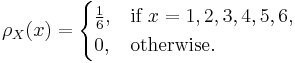
$\rho_Y(y) = \begin{cases}\frac{1}{2},& \text{if }y=0,\\ \frac{1}{2},& \text{if }y=1,\\ 0,& \text{otherwise} .\end{cases}$

A random variable can also be used to describe the process of rolling a fair die and the possible outcomes. The most obvious representation is to take the set {1, 2, 3, 4, 5, 6} as the sample space, defining the random variable X as the number rolled. In this case,

$X = \begin{cases}1,& \text{if a 1 is rolled} ,\\ 2,& \text{if a 2 is rolled} ,\\ 3,& \text{if a 3 is rolled} ,\\ 4,& \text{if a 4 is rolled} ,\\ 5,& \text{if a 5 is rolled} ,\\ 6,& \text{if a 6 is rolled} .\end{cases}$

$\rho_X(x) = \begin{cases}\frac{1}{6},& \text{if }x=1,2,3,4,5,6,\\ 0,& \text{otherwise} .\end{cases}$

An example of a continuous random variable would be one based on a spinner that can choose a horizontal direction. Then the values taken by the random variable are directions. We could represent these directions by North West, East South East, etc. However, it is commonly more convenient to map the sample space to a random variable which takes values which are real numbers. This can be done, for example, by mapping a direction to a bearing in degrees clockwise from North. The random variable then takes values which are real numbers from the interval [0, 360), with all parts of the range being "equally likely". In this case, X = the angle spun. Any real number has probability zero of being selected, but a positive probability can be assigned to any range of values. For example, the probability of choosing a number in [0, 180] is ½. Instead of speaking of a probability mass function, we say that the probability density of X is 1/360. The probability of a subset of [0, 360) can be calculated by multiplying the measure of the set by 1/360. In general, the probability of a set for a given continuous random variable can be calculated by integrating the density over the given set.

An example of a random variable of mixed type would be based on an experiment where a coin is flipped and the spinner is spun only if the result of the coin toss is heads. If the result is tails, X = −1; otherwise X = the value of the spinner as in the preceding example. There is a probability of ½ that this random variable will have the value −1. Other ranges of values would have half the probability of the last example.

Non-real-valued form

Very commonly a random variable takes values which are numbers. This is by no means always so; one can consider random variables of any type. This often includes vector-valued random variables or complex-valued random variables, but in general can include arbitrary types such as sequences, sets, shapes, manifolds, matrices, and functions.

Formal definition

Let (Ω, ℱ, P) be a probability space, and (E, ℰ) a measurable space. Then an (E, ℰ)-valued random variable is a function X: Ω→E, which is (ℱ, ℰ)-measurable. That is, such function that for every subset B ∈ ℰ, its preimage lies in ℱ: X⁻¹(B) ∈ ℱ, where X⁻¹(B) = {ω: X(ω) ∈ B}.^[2]

When E is a topological space, then the most common choice for the σ-algebra ℰ is to take it equal to the Borel σ-algebra ℬ(E), which is the σ-algebra generated by the collection of all open sets in E. In such case the (E, ℰ)-valued random variable is called the E-valued random variable. Moreover, when space E is the real line ℝ, then such real-valued random variable is called simply the random variable.

The meaning of this definition is following: suppose (Ω, ℱ, P) is the underlying probability space, whereas we want to consider a probability space based on the space E with σ-algebra ℰ. In order to turn the pair (E, ℰ) into a probability space, we need to equip it with some probability function, call it Q. This function would have to assign the probability to each set B in ℰ. If X is some function from Ω to E, then it is natural to postulate that the probability of B must be the same as the probability of its preimage in Ω: Q(B) = P(X⁻¹(B)). In order for this formula to be meaningful, X⁻¹(B) must lie in ℱ, since the probability function P is defined only on ℱ. And this is exactly what the definition of the random variable requires: that X⁻¹(B) ∈ ℱ for every B ∈ ℰ.

Real-valued random variables

In this case the observation space is the real numbers with a suitable measure. Recall, $(\Omega, \mathcal{F}, P)$ is the probability space. For real observation space, the function $X: \Omega \rightarrow \mathbb{R}$ is a real-valued random variable if

$\{ \omega�: X(\omega) \le r \} \in \mathcal{F} \qquad \forall r \in \mathbb{R}$

This definition is a special case of the above because $\{(-\infty, r]: r \in \R\}$ generates the Borel sigma-algebra on the real numbers, and it is enough to check measurability on a generating set. (Here we are using the fact that $\{ \omega�: X(\omega) \le r \} = X^{-1}((-\infty, r])$ .)

Distribution functions of random variables

Associating a cumulative distribution function (CDF) with a random variable is a generalization of assigning a value to a variable. If the CDF is a (right continuous) Heaviside step function then the variable takes on the value at the jump with probability 1. In general, the CDF specifies the probability that the variable takes on particular values.

If a random variable $X: \Omega \to \mathbb{R}$ defined on the probability space $(\Omega, \mathcal{F}, P)$ is given, we can ask questions like "How likely is it that the value of $X$ is bigger than 2?". This is the same as the probability of the event $\{ \omega�: X(\omega) > 2 \}\,\!$ which is often written as $P(X > 2)\,\!$ for short, and easily obtained since $P(X > 2)=1-P(X \le 2)$

Recording all these probabilities of output ranges of a real-valued random variable X yields the probability distribution of X. The probability distribution "forgets" about the particular probability space used to define X and only records the probabilities of various values of X. Such a probability distribution can always be captured by its cumulative distribution function

$F_X(x) = \operatorname{P}(X \le x)$

and sometimes also using a probability density function. In measure-theoretic terms, we use the random variable X to "push-forward" the measure P on Ω to a measure dF on R. The underlying probability space Ω is a technical device used to guarantee the existence of random variables, and sometimes to construct them. In practice, one often disposes of the space Ω altogether and just puts a measure on R that assigns measure 1 to the whole real line, i.e., one works with probability distributions instead of random variables.

Moments

The probability distribution of a random variable is often characterised by a small number of parameters, which also have a practical interpretation. For example, it is often enough to know what its "average value" is. This is captured by the mathematical concept of expected value of a random variable, denoted E[X], and also called the first moment. In general, E[f(X)] is not equal to f(E[X]). Once the "average value" is known, one could then ask how far from this average value the values of X typically are, a question that is answered by the variance and standard deviation of a random variable.

Mathematically, this is known as the (generalised) problem of moments: for a given class of random variables X, find a collection {f_i} of functions such that the expectation values E[f_i(X)] fully characterise the distribution of the random variable X.

Functions of random variables

If we have a random variable $X,\!$ on $\Omega \,\!$ and a Borel measurable function $g: \mathbb{R} \rightarrow \mathbb{R}$ , then $Y = g(X)\,\!$ will also be a random variable on $\Omega\,\!$ , since the composition of measurable functions is also measurable. (However, this is not true if $g$ is Lebesgue measurable.) The same procedure that allowed one to go from a probability space $(\Omega, P)\,\!$ to $(\mathbb{R}, dF_{X})$ can be used to obtain the distribution of $Y\,\!$ . The cumulative distribution function of $Y\,\!$ is

$F_Y(y) = \operatorname{P}(g(X) \le y).$

If function g is invertible, i.e. g^-1 exists, and increasing, then the previous relation can be extended to obtain

$F_Y(y) = \operatorname{P}(g(X) \le y) = \operatorname{P}(X \le g^{-1}(y)) = F_X(g^{-1}(y))$

and, again with the same hypotheses of invertibility of g, assuming also differentiability, we can find the relation between the probability density functions by differentiating both sides with respect to y, in order to obtain

$f_Y(y) = f_X(g^{-1}(y)) \left| \frac{d g^{-1}(y)}{d y} \right|$ .

If there is no invertibility of g but each y admits at most a countable number of roots (i.e. a finite, or countably infinite, number of x_i such that y = g(x_i)) then the previous relation between the probability density functions can be generalized with

$f_Y(y) = \sum_{i} f_X(g_{i}^{-1}(y)) \left| \frac{d g_{i}^{-1}(y)}{d y} \right|$

where x_i = g_i^-1(y). The formulas for densities do not demand g to be increasing.

Example 1

Let X be a real-valued, continuous random variable and let Y = X².

$F_Y(y) = \operatorname{P}(X^2 \le y).$

If y < 0, then P(X² ≤ y) = 0, so

$F_Y(y) = 0\qquad\hbox{if}\quad y < 0.$

If y ≥ 0, then

$\operatorname{P}(X^2 \le y) = \operatorname{P}(|X| \le \sqrt{y}) = \operatorname{P}(-\sqrt{y} \le X \le \sqrt{y}),$

$F_Y(y) = F_X(\sqrt{y}) - F_X(-\sqrt{y})\qquad\hbox{if}\quad y \ge 0.$

Example 2

Suppose $\scriptstyle X$ is a random variable with a cumulative distribution

$F_{X}(x) = P(X \leq x) = \frac{1}{(1 + e^{-x})^{\theta}}$

where $\scriptstyle \theta > 0$ is a fixed parameter. Consider the random variable $\scriptstyle Y = \mathrm{log}(1 + e^{-X}).$ Then,

$F_{Y}(y) = P(Y \leq y) = P(\mathrm{log}(1 + e^{-X}) \leq y) = P(X > -\mathrm{log}(e^{y} - 1)).\,$

The last expression can be calculated in terms of the cumulative distribution of $X,$ so

$F_{Y}(y) = 1 - F_{X}(-\mathrm{log}(e^{y} - 1)) \,$

$= 1 - \frac{1}{(1 + e^{\mathrm{log}(e^{y} - 1)})^{\theta}}$

$= 1 - \frac{1}{(1 + e^{y} - 1)^{\theta}}$

$= 1 - e^{-y \theta}.\,$

Equivalence of random variables

There are several different senses in which random variables can be considered to be equivalent. Two random variables can be equal, equal almost surely, equal in mean, or equal in distribution.

In increasing order of strength, the precise definition of these notions of equivalence is given below.

Equality in distribution

If the sample space is a subset of the real line a possible definition is that random variables X and Y are equal in distribution if they have the same distribution functions:

$\operatorname{P}(X \le x) = \operatorname{P}(Y \le x)\quad\hbox{for all}\quad x.$

Two random variables having equal moment generating functions have the same distribution. This provides, for example, a useful method of checking equality of certain functions of i.i.d. random variables. However, the moment generating function exists only for distributions that are good enough.

Almost sure equality

Two random variables X and Y are equal almost surely if, and only if, the probability that they are different is zero:

$\operatorname{P}(X \neq Y) = 0.$

For all practical purposes in probability theory, this notion of equivalence is as strong as actual equality. It is associated to the following distance:

$d_\infty(X,Y)=\mathrm{ess } \sup_\omega|X(\omega)-Y(\omega)|,$

where "ess sup" represents the essential supremum in the sense of measure theory.

Equality

Finally, the two random variables X and Y are equal if they are equal as functions on their probability space, that is,

$X(\omega)=Y(\omega)\qquad\hbox{for all}\quad\omega.$

Convergence

Much of mathematical statistics consists in proving convergence results for certain sequences of random variables; see for instance the law of large numbers and the central limit theorem.

There are various senses in which a sequence (X_n) of random variables can converge to a random variable X. These are explained in the article on convergence of random variables.

References

↑ Rice, John (1999). Mathematical Statistics and Data Analysis. Duxbury Press. ISBN 0534209343.
↑ Fristedt & Gray (1996, page 11)

Literature

Fristedt, Bert; Gray, Lawrence (1996). A modern approach to probability theory. Boston: Birkhäuser. ISBN 3-7643-3807-5.
Kallenberg, O., Random Measures, 4th edition. Academic Press, New York, London; Akademie-Verlag, Berlin (1986). MR0854102 ISBN 0-12-394960-2
Kallenberg, O., Foundations of Modern Probability, 2nd edition. Springer-Verlag, New York, Berlin, Heidelberg (2001). ISBN 0-387-95313-2
Papoulis, Athanasios 1965 Probability, Random Variables, and Stochastic Processes. McGraw–Hill Kogakusha, Tokyo, 9th edition, ISBN 0-07-119981-0.

This article incorporates material from Random variable on PlanetMath, which is licensed under the Creative Commons Attribution/Share-Alike License.

Statistics

Descriptive statistics

Continuous data

Location	Mean (Arithmetic, Geometric, Harmonic) · Median · Mode

Dispersion	Range · Standard deviation · Coefficient of variation · Percentile · Interquartile range

Shape	Variance · Skewness · Kurtosis · Moments · L-moments

Count data

Index of dispersion

Summary tables

Grouped data · Frequency distribution · Contingency table

Dependence

Pearson product-moment correlation · Rank correlation (Spearman's rho, Kendall's tau) · Partial correlation · Scatter plot

Statistical graphics

Bar chart · Biplot · Box plot · Control chart · Correlogram · Forest plot · Histogram · Q-Q plot · Run chart · Scatter plot · Stemplot · Radar chart

Data collection

Designing studies	Effect size · Standard error · Statistical power · Sample size determination

Survey methodology	Sampling · Stratified sampling · Opinion poll · Questionnaire

Controlled experiment	Design of experiments · Randomized experiment · Random assignment · Replication · Blocking · Regression discontinuity · Optimal design

Uncontrolled studies	Natural experiment · Quasi-experiment · Observational study

Statistical inference

Bayesian inference	Bayesian probability · Prior · Posterior · Credible interval · Bayes factor · Bayesian estimator · Maximum posterior estimator

Frequentist inference	Confidence interval · Hypothesis testing · Sampling distribution · Meta-analysis

Specific tests	Z-test (normal) · Student's t-test · F-test · Chi-square test · Pearson's chi-square · Wald test · Mann–Whitney U · Shapiro–Wilk · Signed-rank · Likelihood-ratio

General estimation	Mean-unbiased · Median-unbiased · Maximum likelihood · Method of moments · Minimum distance · Maximum spacing · Density estimation

Correlation and regression analysis

Correlation	Pearson product-moment correlation · Partial correlation · Confounding variable · Coefficient of determination

Regression analysis	Errors and residuals · Regression model validation · Mixed effects models · Simultaneous equations models

Linear regression	Simple linear regression · Ordinary least squares · General linear model · Bayesian regression

Non-standard predictors	Nonlinear regression · Nonparametric · Semiparametric · Isotonic · Robust

Generalized linear model	Exponential families · Logistic (Bernoulli) · Binomial · Poisson

Formal analyses	Analysis of variance (ANOVA) · Analysis of covariance · Multivariate ANOVA

Data analyses and models for other specific data types


Multivariate statistics	Multivariate regression · Principal components · Factor analysis · Cluster analysis · Copulas

Time series analysis	Decomposition · Trend estimation · Box–Jenkins · ARMA models · Spectral density estimation

Survival analysis	Survival function · Kaplan–Meier · Logrank test · Failure rate · Proportional hazards models · Accelerated failure time model

Categorical data	McNemar's test · Cohen's kappa

Applications

Engineering statistics	Methods engineering · Probabilistic design · Process & Quality control · Reliability · System identification

Environmental statistics	Geostatistics · Climatology

Medical statistics	Epidemiology · Clinical trial · Clinical study design

Social statistics	Actuarial science · Population · Demography · Census · Psychometrics · Official statistics · Crime statistics

Category · Portal · Outline · Index